import numpy as np
import matplotlib.pyplot as plt10 Regression
Given a dataset with inputs \(X\) and output \(Y\), a regression model is a model \[\hat{Y} = \hat{f}(X)\] which optimizes parameters of \(\hat{f}\) such that the squared error between the model and observations is minimized. In other words, regression is the process of finding a “best-fit” function \(\hat{f}\) to your data.
This section utilizes NumPy and Pyplot:
10.1 Polynomial Regression
NumPy’s polyfit function determines optimized parameters for a polynomial to fit the given data \(X\) and \(Y\), along with the specified degree of the polynomial. With those parameters, the polyval function evaluates polynomials which is useful for model prediction and visualization.
Given the data:
X = np.array([1,2,3,4,5, 6, 7, 8, 9])
Y = np.array([8,6,5,6,9,12,15,16,16])
we fit polynomials of desired degree with polyfit:
| Description | Model | Python |
|---|---|---|
| Constant | \(\hat{Y}=\beta_0\) | params = np.polyfit(X,Y,0) |
| Linear | \(\hat{Y}=\beta_0 + \beta_1 X\) | params = np.polyfit(X,Y,1) |
| Quadratic | \(\hat{Y}=\beta_0 + \beta_1 X + \beta_2 X^2\) | params = np.polyfit(X,Y,2) |
| Cubic | \(\hat{Y}=\beta_0 + \beta_1 X + \beta_2 X^2 + \beta_3 X^3\) | params = np.polyfit(X,Y,3) |
The polyfit function returns the parameters of the model. Confusingly, it returns the parameters in reverse order from \(\beta_n\) down to \(\beta_0\).
10.1.1 Linear Regression
A complete linear regression looks like this:
params = np.polyfit(X, Y, 1)
print( params )
[1.46666667 3. ]That is the slope of \(\beta_1=1.46\) and \(y\)-intercept of \(\beta_0=3\). Any polynomial can be evaluated for given \(X\) values with polyval, which is useful for making model predictions and plotting:
# Plot the data
plt.scatter(X, Y)

# Plot the regression
Y_hat = np.polyval(params, X)
plt.plot(X, Y_hat )

plt.xlabel('x')
plt.ylabel('y')
plt.title('Linear Regression')
plt.show()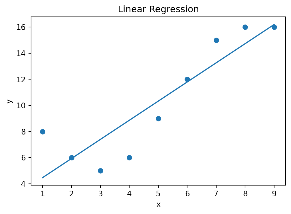
Model predictions can be calculated for individual input values:
# Input value
x1 = 3.5

# Model prediction
y1 = np.polyval(params, x1)
Residual error is the difference between the observed data \((x_i, y_i)\) and the model prediction \((x_i, \hat{y}_i)\), \[ e_i = y_i - \hat{y}_i \] The residuals for our linear model are calculated and visualized with:
Y_hat = np.polyval(params, X)
residuals = Y - Y_hat

plt.axhline(0, color='black')
plt.scatter(X, residuals)
plt.xlabel('x')
plt.title('Residual Error')
plt.show()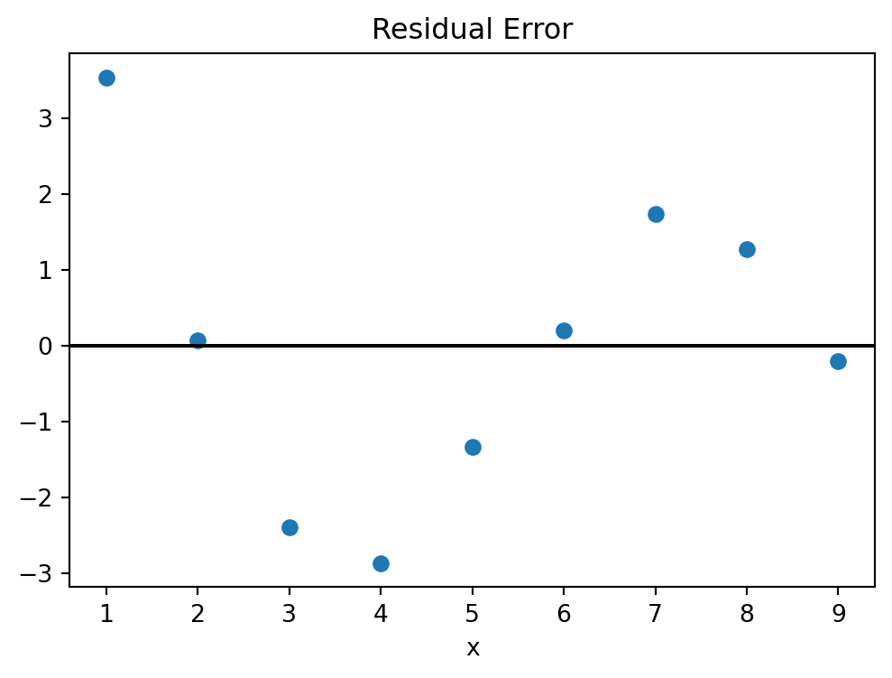
The structure of residual error can give us information about how well the model fits the data. Here, there appears to be a wave-like signal our model has failed to capture. Roughly, we want to see residual error that looks like noise.
10.1.2 Higher-Order Polynomials
Let us look at multiple polynomial models simultaneously:
# Fit models to the data
line_params = np.polyfit(X, Y, 1)
quad_params = np.polyfit(X, Y, 2)
cube_params = np.polyfit(X, Y, 3)

# Plot the data
plt.scatter(X, Y)

# Plot the models
x = np.linspace(1,9,50)
plt.plot( x, np.polyval(line_params, x) )
plt.plot( x, np.polyval(quad_params, x) )
plt.plot( x, np.polyval(cube_params, x) )

plt.xlabel('x')
plt.ylabel('y')
plt.show()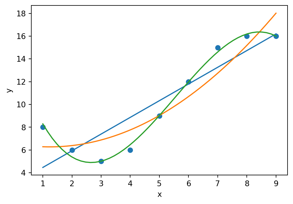
10.2 Model Regression
Exercises
Find the parameters of the linear regression of the model \(\hat{Y}=\beta_0+\beta_1 X\) on the following data:
\(x\) -4 -1 0 2 3 5 6 7 9 \(y\) 22 19 15 16 15 19 19 20 22 Given the linear model \(\hat{Y}=\beta_0+\beta_1 X\) for the above data, find:
- The residual errors \(e_i = y_i - \hat{y}_i\)
- The sum of squared errors \(\sum_{i=1}^{n} e_{i}^{2}\)
- The mean-squared error \(\frac{1}{n}\sum_{i=1}^{n} e_{i}^{2}\)
Plot the data and the linear model.
Repeat the above for a quadratic model \(\hat{Y}=\beta_0+\beta_1 X + \beta_2 X^2\).